Prioritizing alerts in ArcGIS Pro, QGIS and Python

Abstract

Grouping neighboring alerts, measuring the area, count, recency and speed of each group and turning it all into a priority score. With the original script’s parameters, the 11 top-priority groups hold almost 40% of the year’s alert area.

Level Advanced Reading 14 min Data October 2026 Programs ArcGIS

With hundreds of alerts a month, enforcement teams need to decide where to start. The script I used did this in four steps: put alerts that are close to each other into a group, measure each group, turn the measurements into indices from 0 to 1 and add them up with weights.

Course module 5 (in Portuguese) does a version of this in SQL, step by step. Here is the original script’s logic, with the same parameters, in each program.

Map of the Novo Progresso region with protected areas in light green and groups of alerts colored: very low in light yellow, low in yellow, medium in orange, high in red and very high in dark red. The 11 very-high-priority groups are scattered across the study area, several of them on the edges of protected areas. — Groups of alerts from the last year, colored by priority.

The logic

flowchart LR
    A["Alerts from<br/>the last year"] --> B["Group neighbors<br/>60 m / 800 m"]
    B --> C["Group measures:<br/>area, count,<br/>recency, speed"]
    C --> D["Indices 0 to 1<br/>(with limits)"]
    D --> E["Weighted score<br/>0.2 / 0.2 / 0.2 / 0.4"]
    E --> F["Class:<br/>Very Low to<br/>Very High"]

From alert to group to score

Group measure	How it is computed	Limits: clear-cut	Limits: mining	Weight
Area	sum of the alerts’ area (ha)	3 to 30 ha	0.1 to 5 ha	0.2
Count	number of alerts in the group	1 to 4	1 to 10	0.2
Recency	days between the group’s newest alert and the reference date	−365 to −14 days	−365 to −14 days	0.2
Speed	area ÷ days since the group’s first alert (ha/day)	0.1 to 0.5	0.00057 to 0.1	0.4

Grouping: alerts within 60 m of each other (clear-cut) or 800 m (mining, which spreads along rivers) become a single group.
Index with limits: below the minimum it is 0, above the maximum it is 1, and in between it grows linearly. A group of 30 ha or more already has an area index of 1.
Classes: ≥ 0.95 Very High; ≥ 0.8 High; ≥ 0.6 Medium; ≥ 0.4 Low; below that, Very Low.

Reference date

The original script measured recency up to today. Here, the reference is the date of the newest alert (2026-10-16), so the result does not change just because the script ran on another day. For daily use, switch to today’s date.

The code

Data: the deter layer of the articles’ GeoPackage (how to download). The original script used alerts from the Brasil MAIS program, which are restricted to government agencies; DETER works the same way. Names in Portuguese: grupos = groups, tipo = type (corte_raso = clear-cut, mineracao = mining), qtde = count, tempo = recency, velo = speed, primeiro/ultimo = first/last, indice = score, prioridade = priority.

import arcpy
from datetime import timedelta

arcpy.env.overwriteOutput = True
arcpy.env.outputCoordinateSystem = arcpy.SpatialReference(5880)     # meters
gpkg = r"C:\dados\artigos.gpkg"
gdb = r"C:\dados\resultados.gdb"

PARAM = {
    "corte_raso": dict(dist=60, area=(3, 30), qtde=(1, 4), velo=(0.1, 0.5)),
    "mineracao":  dict(dist=800, area=(0.1, 5), qtde=(1, 10), velo=(0.00057, 0.1)),
}

def norm(valor, limites):
    a, b = limites
    return min(1, max(0, (valor - a) / (b - a)))

def classe(x):
    for limite, nome in [(0.95, "Very High"), (0.8, "High"), (0.6, "Medium"), (0.4, "Low")]:
        if x >= limite:
            return nome
    return "Very Low"

# 1 and 2. Alerts from the last year, repaired, with area and type
deter = arcpy.management.CopyFeatures(gpkg + r"\main.deter", r"memory\deter")
ref = max(r[0] for r in arcpy.da.SearchCursor(deter, ["view_date"]))
corte = (ref - timedelta(days=365)).strftime("%Y-%m-%d")
alertas = arcpy.analysis.Select(
    deter, r"memory\alertas",
    "classname IN ('DESMATAMENTO_CR', 'DESMATAMENTO_VEG', 'MINERACAO') "
    f"AND view_date > timestamp '{corte} 00:00:00'")
arcpy.management.RepairGeometry(alertas)
arcpy.management.CalculateGeometryAttributes(
    alertas, [["area_ha", "AREA_GEODESIC"]], area_unit="HECTARES")
arcpy.management.CalculateField(
    alertas, "tipo", "'mineracao' if !classname! == 'MINERACAO' else 'corte_raso'",
    "PYTHON3", field_type="TEXT")

tabelas = []
for tipo, p in PARAM.items():
    a = arcpy.analysis.Select(alertas, rf"memory\a_{tipo}", f"tipo = '{tipo}'")

    # 3. Group: buffer of half the distance, dissolve everything and split the parts
    grupos = arcpy.analysis.PairwiseBuffer(a, rf"memory\buf_{tipo}",
                                           f"{p['dist'] / 2} Meters", dissolve_option="ALL")
    grupos = arcpy.management.MultipartToSinglepart(grupos, rf"memory\grupos_{tipo}")
    arcpy.management.CalculateField(grupos, "cluster", f"'{tipo}_' + str(!OBJECTID!)",
                                    "PYTHON3", field_type="TEXT")
    a = arcpy.analysis.SpatialJoin(a, grupos, rf"memory\aj_{tipo}", "JOIN_ONE_TO_ONE",
                                   "KEEP_COMMON", match_option="INTERSECT")

    # 4. Measures of each group
    t = arcpy.analysis.Statistics(a, rf"memory\t_{tipo}",
                                  [["area_ha", "SUM"], ["gid", "COUNT"],
                                   ["view_date", "MIN"], ["view_date", "MAX"]], "cluster")

    # 5. Indices, score and class
    for campo, tipo_campo in [("tempo", "LONG"), ("velo", "DOUBLE"),
                              ("indice", "DOUBLE"), ("prioridade", "TEXT"), ("tipo", "TEXT")]:
        arcpy.management.AddField(t, campo, tipo_campo)
    campos = ["SUM_area_ha", "COUNT_gid", "MIN_view_date", "MAX_view_date",
              "tempo", "velo", "indice", "prioridade", "tipo"]
    with arcpy.da.UpdateCursor(t, campos) as cursor:
        for area, qtde, primeiro, ultimo, *_ in cursor:
            tempo = (ultimo - ref).days
            velo = area / max(1, (ref - primeiro).days)
            indice = (0.2 * norm(area, p["area"]) + 0.2 * norm(qtde, p["qtde"])
                      + 0.2 * norm(tempo, (-365, -14)) + 0.4 * norm(velo, p["velo"]))
            cursor.updateRow([area, qtde, primeiro, ultimo, tempo, velo, indice,
                              classe(indice), tipo])
    arcpy.management.JoinField(grupos, "cluster", t, "cluster")
    tabelas.append(grupos)

arcpy.management.Merge(tabelas, gdb + r"\priorizacao_grupos")

Note

The original script grouped with Aggregate Polygons (cartography.AggregatePolygons), which is only available with an Advanced license. A dissolved buffer of half the distance gives the same groups and works with a Basic license.

import processing
G = "C:/dados/artigos.gpkg"

PARAM = {
    "corte_raso": dict(dist=60, area=(3, 30), qtde=(1, 4), velo=(0.1, 0.5)),
    "mineracao":  dict(dist=800, area=(0.1, 5), qtde=(1, 10), velo=(0.00057, 0.1)),
}

def rodar(alg, **p):
    p.setdefault("OUTPUT", "memory:")
    return processing.run(alg, p)["OUTPUT"]

def norm(campo, limites):
    """QGIS expression: normalizes between the limits and clamps at 0 and 1."""
    a, b = limites
    return f'clamp(0, ("{campo}" - {a}) / ({b} - {a}), 1)'

# 1. Reference date (the newest alert) and alerts from the last year
fonte = QgsVectorLayer(f"{G}|layername=deter", "deter", "ogr")
ref = fonte.maximumValue(fonte.fields().indexOf("view_date"))
corte = ref.addDays(-365).toString("yyyy-MM-dd")
ref = ref.toString("yyyy-MM-dd")
alertas = rodar("native:extractbyexpression", INPUT=fonte, EXPRESSION=
                "classname IN ('DESMATAMENTO_CR', 'DESMATAMENTO_VEG', 'MINERACAO') "
                f"AND view_date > '{corte}'")

# 2. Repair, convert to meters, area in hectares and type
alertas = rodar("native:fixgeometries", INPUT=alertas)
alertas = rodar("native:removenullgeometries", INPUT=alertas, REMOVE_EMPTY=True)
alertas = rodar("native:reprojectlayer", INPUT=alertas, TARGET_CRS="EPSG:5880")
alertas = rodar("native:fieldcalculator", INPUT=alertas, FIELD_NAME="area_ha", FIELD_TYPE=0,
                FIELD_PRECISION=4,
                FORMULA="area(transform($geometry, 'EPSG:5880', 'ESRI:102033')) / 10000")
alertas = rodar("native:fieldcalculator", INPUT=alertas, FIELD_NAME="tipo", FIELD_TYPE=2,
                FORMULA="if(classname = 'MINERACAO', 'mineracao', 'corte_raso')")

partes = []
for tipo, p in PARAM.items():
    a = rodar("native:extractbyattribute", INPUT=alertas, FIELD="tipo", OPERATOR=0, VALUE=tipo)

    # 3. Group: buffer of half the distance, dissolve and split the parts
    grupos = rodar("native:buffer", INPUT=a, DISTANCE=p["dist"] / 2, DISSOLVE=True)
    grupos = rodar("native:multiparttosingleparts", INPUT=grupos)
    grupos = rodar("native:fieldcalculator", INPUT=grupos, FIELD_NAME="cluster", FIELD_TYPE=2,
                   FORMULA=f"'{tipo}_' || to_string(@row_number)")
    a = rodar("native:joinattributesbylocation", INPUT=a, JOIN=grupos, PREDICATE=[0],
              JOIN_FIELDS=["cluster"], METHOD=1)

    # 4. Measures of each group
    c = rodar("native:aggregate", INPUT=a, GROUP_BY='"cluster"', AGGREGATES=[
        {"aggregate": "first_value", "input": '"cluster"', "name": "cluster", "type": 10,
         "length": 30, "precision": 0},
        {"aggregate": "first_value", "input": '"tipo"', "name": "tipo", "type": 10,
         "length": 12, "precision": 0},
        {"aggregate": "sum", "input": '"area_ha"', "name": "area_ha", "type": 6,
         "length": 0, "precision": 4},
        {"aggregate": "count", "input": '"gid"', "name": "qtde", "type": 2,
         "length": 0, "precision": 0},
        {"aggregate": "minimum", "input": '"view_date"', "name": "primeiro", "type": 14,
         "length": 0, "precision": 0},
        {"aggregate": "maximum", "input": '"view_date"', "name": "ultimo", "type": 14,
         "length": 0, "precision": 0}])
    c = rodar("native:fieldcalculator", INPUT=c, FIELD_NAME="tempo", FIELD_TYPE=1,
              FORMULA=f"-day(to_date('{ref}') - \"ultimo\")")
    c = rodar("native:fieldcalculator", INPUT=c, FIELD_NAME="velo", FIELD_TYPE=0,
              FIELD_PRECISION=5,
              FORMULA=f"\"area_ha\" / max(1, day(to_date('{ref}') - \"primeiro\"))")

    # 5. Weighted score and class
    c = rodar("native:fieldcalculator", INPUT=c, FIELD_NAME="indice", FIELD_TYPE=0,
              FIELD_PRECISION=4, FORMULA=(
                  f"0.2 * {norm('area_ha', p['area'])} + 0.2 * {norm('qtde', p['qtde'])} + "
                  f"0.2 * {norm('tempo', (-365, -14))} + 0.4 * {norm('velo', p['velo'])}"))
    c = rodar("native:fieldcalculator", INPUT=c, FIELD_NAME="prioridade", FIELD_TYPE=2,
              FORMULA="CASE WHEN indice >= 0.95 THEN 'Very High' WHEN indice >= 0.8 THEN "
                      "'High' WHEN indice >= 0.6 THEN 'Medium' WHEN indice >= 0.4 THEN 'Low' "
                      "ELSE 'Very Low' END")
    partes.append(c)

clusters = rodar("native:mergevectorlayers", LAYERS=partes, CRS="EPSG:5880",
                 OUTPUT="C:/dados/priorizacao_qgis.gpkg")
resumo = rodar("qgis:statisticsbycategories", INPUT=clusters,
               CATEGORIES_FIELD_NAME=["tipo", "prioridade"])
for f in resumo.getFeatures():
    print(f["tipo"], f["prioridade"], f["count"])

Grouping uses the same idea as in ArcGIS: two alerts within 60 m of each other have 30 m buffers that touch, and Dissolve merges them. The clamp, day and max functions in the expressions do the rest.

ST_ClusterDBSCAN does the grouping directly: with minpoints = 1, it joins every geometry within eps meters of another one in the group, just like Aggregate Polygons.

-- Parameters of the original script
DROP TABLE IF EXISTS artigos.prior_param;
CREATE TABLE artigos.prior_param (tipo text PRIMARY KEY, dist numeric,
    area_min numeric, area_max numeric, qtde_min numeric, qtde_max numeric,
    velo_min numeric, velo_max numeric);
INSERT INTO artigos.prior_param VALUES
    ('corte_raso', 60, 3, 30, 1, 4, 0.1, 0.5),
    ('mineracao', 800, 0.1, 5, 1, 10, 0.00057, 0.1);

-- Normalization with limits: below the minimum = 0, above the maximum = 1
CREATE OR REPLACE FUNCTION artigos.normalizar(valor numeric, minimo numeric, maximo numeric)
RETURNS numeric LANGUAGE sql IMMUTABLE AS
$$ SELECT least(1, greatest(0, (valor - minimo) / (maximo - minimo))) $$;

DROP TABLE IF EXISTS artigos.prior_clusters;
CREATE TABLE artigos.prior_clusters AS
WITH ref AS (SELECT max(view_date) AS d FROM artigos.deter),
alertas AS (                                  -- 1 and 2. last year, repaired, in meters
    SELECT a.gid, a.view_date,
           CASE WHEN a.classname = 'MINERACAO' THEN 'mineracao' ELSE 'corte_raso' END AS tipo,
           ST_Transform(ST_CollectionExtract(ST_MakeValid(a.geom), 3), 5880) AS geom
    FROM artigos.deter a, ref
    WHERE a.classname IN ('DESMATAMENTO_CR', 'DESMATAMENTO_VEG', 'MINERACAO')
      AND a.view_date > ref.d - 365
),
agrupados AS (                                -- 3. alerts within 60 m (or 800 m) = same group
    SELECT *, (ST_Area(ST_Transform(geom, 4674)::geography) / 10000)::numeric AS area_ha,
           CASE tipo
               WHEN 'mineracao' THEN ST_ClusterDBSCAN(geom, 800, 1) OVER (PARTITION BY tipo)
               ELSE ST_ClusterDBSCAN(geom, 60, 1) OVER (PARTITION BY tipo)
           END AS cluster
    FROM alertas
    WHERE NOT ST_IsEmpty(geom)
),
medidas AS (                                  -- 4. measures of each group
    SELECT g.tipo, g.cluster, sum(g.area_ha) AS area_ha, count(*) AS qtde,
           max(g.view_date) - ref.d AS tempo,
           sum(g.area_ha) / greatest(1, ref.d - min(g.view_date)) AS velo,
           ST_Union(g.geom) AS geom
    FROM agrupados g, ref
    GROUP BY g.tipo, g.cluster, ref.d
)
SELECT m.*,                                   -- 5. weighted score
       0.2 * artigos.normalizar(m.area_ha, p.area_min, p.area_max)
     + 0.2 * artigos.normalizar(m.qtde, p.qtde_min, p.qtde_max)
     + 0.2 * artigos.normalizar(m.tempo, -365, -14)
     + 0.4 * artigos.normalizar(m.velo, p.velo_min, p.velo_max) AS indice
FROM medidas m
JOIN artigos.prior_param p USING (tipo);

ALTER TABLE artigos.prior_clusters ADD COLUMN prioridade text;
UPDATE artigos.prior_clusters SET prioridade = CASE
    WHEN indice >= 0.95 THEN 'Very High' WHEN indice >= 0.8 THEN 'High'
    WHEN indice >= 0.6 THEN 'Medium' WHEN indice >= 0.4 THEN 'Low' ELSE 'Very Low' END;

SELECT tipo, prioridade, count(*) AS grupos, round(sum(area_ha)) AS area_ha
FROM artigos.prior_clusters
GROUP BY tipo, prioridade
ORDER BY tipo, min(indice) DESC;

import geopandas as gpd
import pandas as pd

# Parameters of the original script: grouping distance, limits of each index and weights
PARAM = {
    "corte_raso": dict(dist=60, area=(3, 30), qtde=(1, 4), velo=(0.1, 0.5)),
    "mineracao":  dict(dist=800, area=(0.1, 5), qtde=(1, 10), velo=(0.00057, 0.1)),
}
TEMPO = (-365, -14)                       # days to the reference date (negative = past)
PESOS = dict(area=0.2, qtde=0.2, tempo=0.2, velo=0.4)
CLASSES = [(0.95, "Very High"), (0.8, "High"), (0.6, "Medium"), (0.4, "Low"), (0, "Very Low")]

# 1. Clear-cut and mining alerts from the last 365 days
deter = gpd.read_file("dados/artigos.gpkg", layer="deter")
deter["view_date"] = pd.to_datetime(deter["view_date"])
ref = deter["view_date"].max()                       # reference date: the newest alert
deter = deter[(deter["view_date"] > ref - pd.Timedelta(days=365))
              & deter["classname"].isin(["DESMATAMENTO_CR", "DESMATAMENTO_VEG", "MINERACAO"])]
deter["tipo"] = deter["classname"].map(lambda c: "mineracao" if c == "MINERACAO" else "corte_raso")

# 2. Repaired geometries, in meters, and area in hectares
deter["geometry"] = deter.make_valid(method="structure", keep_collapsed=False)
deter = deter[~deter.is_empty].to_crs(5880)
deter["area_ha"] = deter.to_crs("ESRI:102033").area / 10_000

def normalizar(valor, limites):
    minimo, maximo = limites
    return ((valor - minimo) / (maximo - minimo)).clip(0, 1)

partes = []
for tipo, p in PARAM.items():
    a = deter[deter["tipo"] == tipo]
    # 3. Group: buffer of half the distance, union and split the parts
    grupos = gpd.GeoDataFrame(geometry=[a.buffer(p["dist"] / 2).union_all()], crs=5880)
    grupos = grupos.explode(index_parts=False).reset_index(drop=True)
    grupos["cluster"] = [f"{tipo}_{i + 1}" for i in range(len(grupos))]
    a = gpd.sjoin(a, grupos, predicate="intersects").drop(columns="index_right")

    # 4. Measures of each group
    c = a.groupby("cluster").agg(area_ha=("area_ha", "sum"), qtde=("gid", "count"),
                                 primeiro=("view_date", "min"), ultimo=("view_date", "max"))
    c["tempo"] = (c["ultimo"] - ref).dt.days                         # 0 = most recent
    c["velo"] = c["area_ha"] / (ref - c["primeiro"]).dt.days.clip(lower=1)

    # 5. Indices from 0 to 1, weighted score and class
    c["indice"] = (PESOS["area"] * normalizar(c["area_ha"], p["area"])
                   + PESOS["qtde"] * normalizar(c["qtde"], p["qtde"])
                   + PESOS["tempo"] * normalizar(c["tempo"], TEMPO)
                   + PESOS["velo"] * normalizar(c["velo"], p["velo"]))
    c["prioridade"] = c["indice"].map(lambda x: next(n for lim, n in CLASSES if x >= lim))
    partes.append(c.assign(tipo=tipo))

clusters = pd.concat(partes)
print("reference date:", ref.date())
print(pd.crosstab(clusters["tipo"], clusters["prioridade"]))
colunas = ["tipo", "area_ha", "qtde", "tempo", "velo", "indice", "prioridade"]
print(clusters.sort_values("indice", ascending=False)[colunas].head(5).round(3))
clusters.to_csv("dados/priorizacao_python.csv")

Checking the result

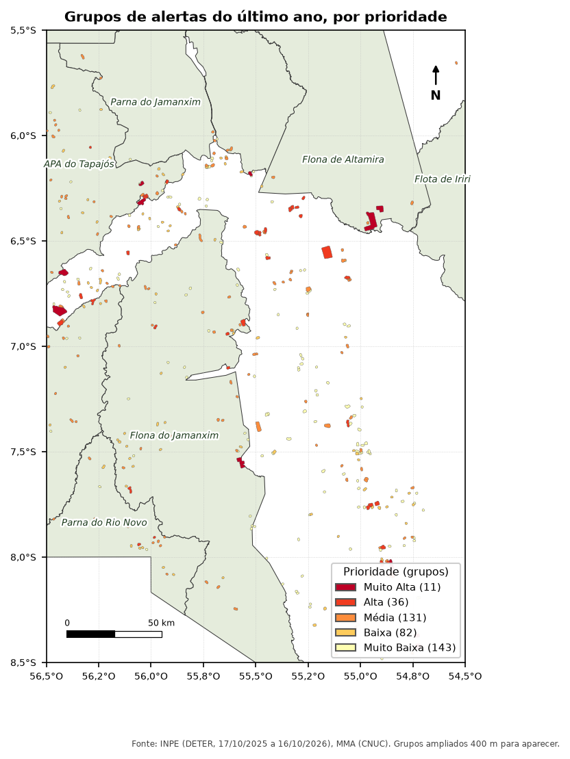
The QGIS, PostGIS and Python versions formed the same groups and gave exactly the same count in each class:

Groups of DETER alerts from 2025-10-17 to 2026-10-16 in the example area.
Priority	Clear-cut groups	Area (ha)	Mining groups	Area (ha)
Very High	11	6,974	0	0
High	29	4,433	7	173
Medium	68	2,150	63	747
Low	26	539	56	489
Very Low	129	1,929	14	110

The 11 very high priority groups add up to almost 7,000 hectares, more than the 129 very low priority groups combined. That is the gain from prioritizing: almost 40% of the year’s alert area is in less than 3% of the groups (11 of 403).

Pitfalls

Distance in degrees

AggregatePolygons and ST_ClusterDBSCAN use the layer’s units. With data in SIRGAS 2000 (degrees), “60” means 60 degrees. Reproject to meters before grouping, as in all the code above.

Speed of an isolated alert

A group with a single alert, detected today, would have a speed of “area ÷ 0 days”. The original divided by the difference up to today; here the divisor has a minimum of 1 day. Choose a rule and write it in the report.

Limits and weights are choices

The limits (30 ha, 4 alerts, 0.5 ha/day…) and the weights came from one team’s experience with one type of alert. They are not official criteria. Test other values and see how the list changes: if the top places do not change, the prioritization is robust.

Updates

2026-10-29: first published, with data from INPE, MMA, IBAMA and SICAR from October 2026.

Versão em português

Reuse

CC BY 4.0

Citation

BibTeX citation:

@misc{alves2026,
  author = {Alves, Hendesson},
  publisher = {Hendesson Alves},
  title = {Prioritizing Alerts in {ArcGIS} {Pro,} {QGIS} and {Python}},
  date = {2026-10-29},
  url = {https://hendesson.github.io/en/articles/12-prioritization-arcgis-qgis.html},
  doi = {10.5281/zenodo.23780268},
  langid = {en},
  abstract = {Grouping neighboring alerts, measuring the area, count,
    recency and speed of each group and turning it all into a priority
    score. With the original script’s parameters, the 11 top-priority
    groups hold almost 40\% of the year’s alert area.}
}

For attribution, please cite this work as:

Alves, Hendesson. 2026. “Prioritizing Alerts in ArcGIS Pro, QGIS and Python.” In Geoprocessing Articles for Environmental Monitoring. Preprint, Hendesson Alves, October 29. https://doi.org/10.5281/zenodo.23780268.